How to generate better images with GAN using Pytorch?

In previous post, we learnt about Variational Autoencoders (VAE) and how they can be used to reconstruct images. But, we also saw the problems with generated images.

In this post, we’ll take a step forward and get to know another neural network architecture called Generative Adversarial Networks (GAN) which are also used to generate images. The word refers “Adversarial” refers to the set of networks which compete against each other in their respective tasks. This method was proposed by Ian Goodfellow and his fellow co-authors in 2014.

Let’s understand the basics in detail.

Basics of GANs

The GAN network consists of two components: Generator and Discriminator.

The Generator takes a random noise vector as an input and generates a set of observations (or image vector) as if they are sampled from the original dataset. Then, the discriminator tries to predict whether the observation comes from the original dataset or not.

Both generator and discriminator perform binary classification underneath. Generator tries to generate an image with an objective of minimizing the probability that the generated image is identified as fake i.e. the fake images should be identified as real by the discriminator. On the other hand, the discriminator tries to maximize the accuracy of predicting a real image as real and fake image as fake.

This fight between generator and discriminator is an iterative process where generator tries to fool discriminator by generating near-real images and discriminator tries to adjust itself to recognise the fake patterns.

You might be wondering isn’t it similar to VAE we learnt in the previous post ? Correct, the generator in GAN does the same job as decoder in VAE. They take a vector (whose observations are sampled from a standard normal distribution) as an input and generates an image.

When we train the network, we must alternate the training process between generator and discriminator, so that both generator and discriminator can continue to compete strongly. Otherwise, one of them will get smarter and the resultant images wouldn’t be sharp or of good quality. This process will overtime make generator network create more realistic images and make discriminators task more difficult to detect real or fake image.

Maybe if its not clear for you, I assure you things will get more clear once you start implementing it step by step as shown below.

Let’s implement a Deep convolutional GAN network (DCGAN) (inspired by this paper) ourselves. We are aiming for deep convolutional network because we already saw in previous blog that fully connected layer network didn’t work well with image generation.

Training a Deep Convolutional GAN from Scratch

We’ll continue using the same Glasses dataset from the VAE post. The dataset contains approx. 5000 images of humans with and without wearing glasses. If you haven’t read the VAE post, you can follow the same steps from the post to read the data, structure the images into separate directories.

Once your dataset is structured into images directory path, lets define the transformations.

from pathlib import Path
import os
import shutil
import torch
from torch import nn
from torch.utils.data import DataLoader
from torchvision import datasets
import torchvision.transforms as T
import torch.nn.functional as F

batch_size=128
transform = T.Compose([
            T.Resize(64),    
            T.RandomHorizontalFlip(),
            T.ColorJitter(brightness=0.1, contrast=0.1),
            T.ToTensor(),
            T.Normalize((0.5, 0.5, 0.5), (0.5, 0.5, 0.5)),
            ])
data = datasets.ImageFolder(root=path/'images', transform=transform)       
loader = torch.utils.data.DataLoader(data, batch_size=batch_size,shuffle=True, num_workers=10, pin_memory=True)

Lets understand the code above:

• We resize the original image size (256) to 64.
• We add data augmentation to increase the training samples. Hence, we add RandomHorizontalFlip, ColorJitter to create images with some variation
• Finally, we normalize the RGB channels of the images.

Lets define our generator architecture. It takes a random vector and generates a vector of the same shape as our images in the dataset.

class Generator(nn.Module):
    def __init__(self):
        super(Generator, self).__init__()
        self.net = nn.Sequential(
            nn.ConvTranspose2d(100, 64 * 8, kernel_size=4, stride=1, padding=0, bias=False),
            nn.BatchNorm2d(64 * 8),
            nn.ReLU(True),

            nn.ConvTranspose2d(64 * 8, 64 * 4, kernel_size=4, stride=2, padding=1, bias=False),
            nn.BatchNorm2d(64 * 4),
            nn.ReLU(True),

            nn.ConvTranspose2d( 64 * 4, 64 * 2, kernel_size=4, stride=2, padding=1, bias=False),
            nn.BatchNorm2d(64 * 2),
            nn.ReLU(True),

            nn.ConvTranspose2d( 64 * 2, 64, kernel_size=4, stride=2, padding=1, bias=False),
            nn.BatchNorm2d(64),
            nn.ReLU(True),

            nn.ConvTranspose2d( 64, 3, kernel_size=4, stride=2, padding=1, bias=False),
            nn.Tanh()
        )

    def forward(self, input):
        return self.net(input)

And the compiled architecture looks like as follows:

Generator(
  (main): Sequential(
    (0): ConvTranspose2d(100, 512, kernel_size=(4, 4), stride=(1, 1), bias=False)
    (1): BatchNorm2d(512, eps=1e-05, momentum=0.1, affine=True, track_running_stats=True)
    (2): ReLU(inplace=True)
    (3): ConvTranspose2d(512, 256, kernel_size=(4, 4), stride=(2, 2), padding=(1, 1), bias=False)
    (4): BatchNorm2d(256, eps=1e-05, momentum=0.1, affine=True, track_running_stats=True)
    (5): ReLU(inplace=True)
    (6): ConvTranspose2d(256, 128, kernel_size=(4, 4), stride=(2, 2), padding=(1, 1), bias=False)
    (7): BatchNorm2d(128, eps=1e-05, momentum=0.1, affine=True, track_running_stats=True)
    (8): ReLU(inplace=True)
    (9): ConvTranspose2d(128, 64, kernel_size=(4, 4), stride=(2, 2), padding=(1, 1), bias=False)
    (10): BatchNorm2d(64, eps=1e-05, momentum=0.1, affine=True, track_running_stats=True)
    (11): ReLU(inplace=True)
    (12): ConvTranspose2d(64, 3, kernel_size=(4, 4), stride=(2, 2), padding=(1, 1), bias=False)
    (13): Tanh()
  )
)

Lets understand the generator block in detail:

• It takes an input vector of length 100.
• The vector goes through several convolutional blocks. Each block consists of ConvTranspose2d, BatchNorm and Relu activation at the end. The main purpose of this block is to keep increasing the size of vector so that the end result is 3 x 64 x 64 image (as our original image).
• nn.ConvTranspose2d helps in increasing the spatial shape of the tensor (starting from 1, then 4, 8,…, 64).
• At the last layer, we use TanH activation function to ensure the range of output if [-1, 1] similar to our normalized input image.

Now, we move to defining the discriminator block.

class Discriminator(nn.Module):
    def __init__(self):
        super(Discriminator, self).__init__()
        self.net = nn.Sequential(
            nn.Conv2d(3, 64, kernel_size=4, stride=2, padding=1, bias=False),
            nn.LeakyReLU(0.2, inplace=True),
            nn.Dropout(0.1),

            nn.Conv2d(64, 64 * 2, kernel_size=4, stride=2, padding=1, bias=False),
            nn.BatchNorm2d(64 * 2),
            nn.LeakyReLU(0.2, inplace=True),
            nn.Dropout(0.1),

            nn.Conv2d(64 * 2, 64 * 4, kernel_size=4, stride=2, padding=1, bias=False),
            nn.BatchNorm2d(64 * 4),
            nn.LeakyReLU(0.2, inplace=True),
            nn.Dropout(0.1),

            nn.Conv2d(64 * 4, 64 * 8, kernel_size=4, stride=2, padding=1, bias=False),
            nn.BatchNorm2d(64 * 8),
            nn.LeakyReLU(0.2, inplace=True),
            nn.Dropout(0.1),

            nn.Conv2d(64 * 8, 1, kernel_size=4, stride=1, padding=0, bias=False),
            nn.Sigmoid()
        )

    def forward(self, input):
        return self.net(input)

Lets walkthrough the discriminator architecture:

• The discriminator receives an image of size 3 x 64 x 64 as an input and predicts probability of the image being fake or real. If its real, the predicted probability should be close to 1 else towards 0.
• It contains multiple convolutional blocks. Here, along with BatchNorm2d, we have introduced LeakyRelu and Dropout layers as well.
• nn.Conv2d helps in decreasing the spatial shape of the tensor (starting from 64, then 32, 24,…, 1).
• LeakyRelu helps in avoiding gradient saturation and ensure the model keeps learning well.
• Dropout ensures that discriminator needs to work harder to predict real or fake. Otherwise, if it predicts easily means the discriminator is over-powering the generator and we won’t get good quality generated images.
• We use Sigmoid activation function at the last layer to ensure predicted probabilities are bounded between 0 and 1.

Now we’ll initialise networks and the loss function, optimizers to use:

netG = Generator().to(device)
netD = Discriminator().to(device)

# Initialize the loss function
criterion = nn.BCELoss()

# set a fix vector used as input to generator
fixed_noise = torch.randn(64, 3, 1, 1, device=device)

real_label = 1
fake_label = 0

# set optimizers for both G and D
optimizerD = optim.Adam(netD.parameters(), lr=1e-4, betas=(0.5, 0.999))
optimizerG = optim.Adam(netG.parameters(), lr=2e-4, betas=(0.5, 0.999))

The important aspects to note are:

• We are using binary cross entropy (BCE) loss to measure the model error.
• The betas plays a significant role in controlling how much past gradients influence the current gradient. It basically keep track of a running mean & variance estimate and updates them as it processes new batch. The value 0.5 controls the influence of mean of gradients. The value 0.999 controls the influence of variance of gradients (on the current sample).
• We set a lower learning rate for generator as compared to discriminator, for the same reason as above, that we don’t to make the discriminator job super easy.

We are almost done setting up the components of the network. Now, we’ll start implementing the training loop. Depending on the device you are using to run this code, it’ll take longer. I am running it on a NVIDIA V100 GPU and it takes around 30 mins to run.

You can see below the training loop is exactly replication the process we discussed above:

# Training Loop
img_list = []
iters = 0
num_epochs = 200

# For each epoch
for epoch in range(num_epochs):

    for i, data in enumerate(loader):

        ############################
        # (1) Train discriminator network: minimize −[log(D(x))+log(1−D(G(z)))]
        ###########################
        ## Train with real data
        netD.zero_grad()
        real_cpu = data[0].to(device)
        batch_size = real_cpu.size(0)

        label = torch.full((batch_size,), real_label, dtype=torch.float, device=device) 
        # Forward pass real batch through D
        output = netD(real_cpu).view(-1)
        # Calculate loss on all-real batch
        errD_real = criterion(output, label)  # = -log(D(x))

        # Calculate gradients using backward pass
        errD_real.backward()
        D_x = output.mean().item()

        ## Train with fake data
        # Generate batch of latent vectors of size 100
        noise = torch.randn(batch_size, 100, 1, 1, device=device)

        # Generate fake image batch with G
        fake = netG(noise)
        # Create a label vector with 0 value
        label.fill_(fake_label)
        # Run forward pass and calculate loss
        output = netD(fake.detach()).view(-1)
        errD_fake = criterion(output, label) # = -log(1 - D(G(z)))

        # Calculate the gradients using backward pass
        errD_fake.backward()
        D_G_z1 = output.mean().item()

        # Compute total error for discriminator
        errD = errD_real + errD_fake
        optimizerD.step()

        ############################
        # (2) Train generator network: minimize - log(D(G(z)))
        ###########################
        netG.zero_grad()
        label.fill_(real_label)  
        output = netD(fake).view(-1)
        # Calculate G's loss based on real labels
        errG = criterion(output, label)
        # Calculate gradients for G
        errG.backward()
        D_G_z2 = output.mean().item()
        # Update G
        optimizerG.step()

        # Output training stats
        if i % 50 == 0:
            print('[%d/%d][%d/%d]\tLoss_D: %.4f\tLoss_G: %.4f\tD(x): %.4f\tD(G(z)): %.4f / %.4f'
                  % (epoch, num_epochs, i, len(loader),
                     errD.item(), errG.item(), D_x, D_G_z1, D_G_z2))

        # Check how the generator is doing by saving G's output on fixed_noise
        if (iters % 10 == 0) or ((epoch == num_epochs-1) and (i == len(loader)-1)):
            with torch.no_grad():
                fake = netG(fixed_noise).detach().cpu()
            img_grid = torchvision.utils.make_grid(fake, normalize=True, padding=2)
            img_list.append(img_grid)

        iters += 1

Lets understand the training loop in detail, this is very important:

• Training discriminator involves two steps:
  • Calculate loss against real data: Here we would like the discriminator model to predict high probabilities (close to 1)
  • Calculate loss against fake data: Here predicting low probability is favorable (low probability of being real)
• Training generator involves following steps:
  • Calculate loss against real data: Here we generate an image and compare it against real labels. This way we make generator update weights in the direction of better image quality.
• Generator updates its weights so that the generated images can be classified as real by the discriminator.

After, I run the training for 200 epochs, we see the following loss curves:

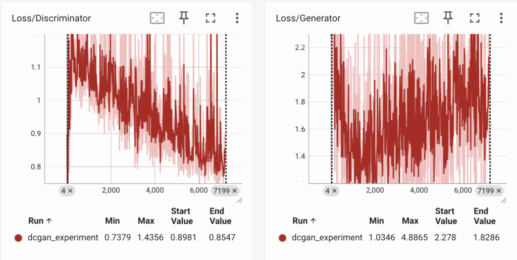
We analyse the following:

• The discriminator is doing quite well since its loss is consistently decreasing. It also means that, for the discriminator its getting quite easy to identify fake and real image (and we don’t want this to happen!)
• The generator loss drops till a point and increases. This means the generator isn’t able to generate high quality fake images. It definitely needs some more work.

Let’s look at some of the generated images:

As you can see, the images aren’t too bad but not too great either. Some of the faces are deformed and distorted. This also confirm with our loss curves. We can definitely do better.

Tips to improve the GAN

You should be proud of yourself and feel happy that you’ve been generate images, the quality above isn’t too bad for the first try. Let’s try to think critically how can be improve it further:

• Discriminator
  • Increase the dropout rate
  • Add noise labels. This means set real_label=0.9, fake_label=0.1
  • Reduce learning rate
  • Simply the network. Eg: Reduce the number of convolutional filters.
  • Reduce frequency of discriminator training. Maybe train it once every two runs of generator.
• Generator
  • Strengthen the network by adding more conv layers.
• Train for longer epochs.

Summary

In this post, we learnt the basics of Generative Adversarial Networks (GAN) and implemented them from scratch using pytorch to generate images. We surely generated better image quality with DCGAN as compared to VAE in the previous post. However, they are still not perfect.

You might be interested to know that besides DCGAN, there also exists Wasserstein GAN, Conditional GAN (CGAN) which fixes the problems with DCGAN and can result in better quality images. We’ll see in the next post how we can further improve our image generation output.

Please feel free to drop your comments, reviews below and share your experience with image generation.